Fuzzy Clustering with NeuroStatX
This tutorial demonstrates how to use the NeuroStatX
Python package for fuzzy clustering in cognitive-behavioral neuroscience. We’ll focus on two use cases:
- Projecting new data onto precomputed fuzzy centroids (e.g., for generalization or replication across cohorts).
- Running fuzzy c-means clustering from scratch to derive data-driven participant profiles (coming soon)
For prediction, the initial clustering approach and validation strategies are detailed in our paper:
Gagnon, A., Gillet, V., Desautels, A.-S., Lepage, J.-F., Baccarelli, A. A., Posner, J., Descoteaux, M., Brunet, M. A., & Takser, L. (2025). Beyond Discrete Classifications: A Computational Approach to the Continuum of Cognition and Behavior in Children. medRxiv. https://doi.org/10.1101/2025.04.14.25325835
Projecting New Participants to Precomputed Centroids
This is useful when you have:
- Fuzzy centroids already derived on a training set (the centroids from the baseline
Adolescent Brain Cognitive Development baseline follow-up are already shipped with
NeuroStatX(Gagnon A et al., 2025)) - New participants data with similar features (e.g., cognitive and behavioral scores).
Why predicting?
Predicting avoids re-fitting clustering and ensures comparability across cohorts. It is also a major advantage when your population does not have enough subjects to derive clusters. You then rely on precomputed centroids from large databases to extract membership values for your new participants.
Requirements for predicting new data into existing centroids.
While the actual prediction is trivial, there is some mandatory assumptions or requirements that need to be met in order to obtain acceptable and sound results.
- If using the centroids from Gagnon A. et al. (2025), your data needs to include the
features [
Internalizing,Externalizing,Stress,VA,EFPS,MEM] in this specific order. - Your data needs to be scaled in order to obtain a mean of 0 with standard deviation of 1. This
step can be performed using
sklearn. - Optionally, if you have access to ABCD data, harmonizing your cognitive and behavioral scores might improve your results.
Viewing test data
NeuroStatX provides a command-line (CLI) tool to predict fuzzy membership values. It also contains
the centroids from the cognitive and behavioral profiles extracted in Gagnon A et al. (2025). Let’s go through
an example with the data/example.csv file. Let’s quickly load it in the python console
and look at its structure before using the CLI script.
from neurostatx.io.loader import DatasetLoader
# Load example.csv from the /data folder.df = DatasetLoader().load_data("data/example.csv")df.get_data().head(5)print(df.get_metadata())
ids Sex Age Int Ext Stress VA EFPS MEM0 PC2VLN Female 10.9 0.853711 -0.155164 0.356608 -0.009190 -0.312745 0.0468851 XL1LON Male 11.6 0.712829 0.893640 0.629955 0.446043 0.422631 0.3369532 F6OQK5 Male 10.7 -0.055407 1.236605 0.501959 -0.657493 -0.451615 -0.3435493 TJWBKZ Male 10.3 -0.172911 -1.340310 -0.582634 0.238857 -0.144028 -0.1788354 KWQW9D Male 10.8 -0.258481 -0.895303 -0.610380 -0.297869 -0.111272 0.016617{'nb_subjects': 50, 'nb_variables': 9}As you can see, we have 50 subjects with 9 features. The first three features are
descriptive variables representing the ID, sex, and age. The next six features are
our features of interest. As you can see, the Int and Ext column do not match
our predefined column name, as long they respect the same order, this should not
be a problem for now. Let’s try this out and see what comes out.
Using the CLI script
To test this out, we will use the PredictFuzzyMembership CLI script. It already
wraps all commands required to predict membership values for new participants.
First, let’s call the help to see which inputs are required.
PredictFuzzyMembership --helpUsage: predictfuzzymembership COMMAND [ARGS] [OPTIONS]
╔═══════════════════════════════════════════════════════════════════════════════════════════════════════════════════════════════════════════════════════════════════════════════════════════════════════╗║ Fuzzy Membership Prediction ║╚═══════════════════════════════════════════════════════════════════════════════════════════════════════════════════════════════════════════════════════════════════════════════════════════════════════╝This script will predict the membership matrix of a dataset using a trained Cmeans model (only the centroids are necessary for the prediction).
╔═══════════════════════════════════════════════════════════════════════════════════════════════════════════════════════════════════════════════════════════════════════════════════════════════════════╗║ Configurations ║╚═══════════════════════════════════════════════════════════════════════════════════════════════════════════════════════════════════════════════════════════════════════════════════════════════════════╝Details regarding the parameters can be seen below. Regarding the --m parameter, it defines the degree of fuzziness of the resulting membership matrix. Using --m 1 will returns crisp clusters, whereas--m >1 will returned more and more fuzzy clusters. It is recommended to use the same m value as used during training.
╔═══════════════════════════════════════════════════════════════════════════════════════════════════════════════════════════════════════════════════════════════════════════════════════════════════════╗║ Example Usage ║╚═══════════════════════════════════════════════════════════════════════════════════════════════════════════════════════════════════════════════════════════════════════════════════════════════════════╝┌─────────────────────────────────────────────────────────────────────────────────────────────── python ────────────────────────────────────────────────────────────────────────────────────────────────┐│ PredictFuzzyMembership --in_dataset dataset.xlsx --in_cntr ││ centroids.xlsx --id_column ID --desc_columns 1 --out_folder ││ predicted_membership_matrix/ --m 2 --error 1e-6 --maxiter 1000 ││ --metric euclidean --verbose --save_parameters --overwrite │└───────────────────────────────────────────────────────────────────────────────────────────────────────────────────────────────────────────────────────────────────────────────────────────────────────┘
╭─ Clustering Options ──────────────────────────────────────────────────────────────────────────────────────────────────────────────────────────────────────────────────────────────────────────────────╮│ M,--m Exponentiation value to apply on the membership function, will determined the degree of fuzziness of the membership matrix. [default: 2] ││ ERROR,--error Error threshold for convergence stopping criterion. [default: 1e-06] ││ MAXITER,--maxiter Maximum number of iterations to perform. [default: 1000] ││ METRIC,--metric Metric to use to compute distance between original points and clusters centroids. [choices: ││ braycurtis,canberra,chebyshev,cityblock,correlation,cosine,dice,euclidean,hamming,jaccard,jensenshannon,kulczynski1,mahalanobis,matching,minkowski,rogerstanimoto,russellrao,… ││ [default: euclidean] ││ PCA,--pca If set, will perform PCA decomposition to 3 components before clustering. [default: False] ││ PCA-MODEL,--pca-model If set, will load a pre-trained PCA model to apply on the dataset. [default: None] │╰───────────────────────────────────────────────────────────────────────────────────────────────────────────────────────────────────────────────────────────────────────────────────────────────────────╯╭─ Commands ────────────────────────────────────────────────────────────────────────────────────────────────────────────────────────────────────────────────────────────────────────────────────────────╮│ --help,-h Display this message and exit. ││ --version Display application version. │╰───────────────────────────────────────────────────────────────────────────────────────────────────────────────────────────────────────────────────────────────────────────────────────────────────────╯╭─ Essential Files Options ─────────────────────────────────────────────────────────────────────────────────────────────────────────────────────────────────────────────────────────────────────────────╮│ * IN-DATASET,--in-dataset Input dataset. [required] ││ * IN-CNTR,--in-cntr Centroid file to use for prediction. Should come from a trained Cmeans model (such as FuzzyClustering). [required] ││ * ID-COLUMN,--id-column Name of the column containing the subject's ID tag. Required for proper handling of IDs and merging multiple datasets. [required] ││ * DESC-COLUMNS,--desc-columns Number of descriptive columns at the beginning of the dataset to exclude in statistics and descriptive tables. [required] ││ OUT-FOLDER,--out-folder Output folder for the predicted membership matrix. │╰───────────────────────────────────────────────────────────────────────────────────────────────────────────────────────────────────────────────────────────────────────────────────────────────────────╯╭─ Optional parameters ─────────────────────────────────────────────────────────────────────────────────────────────────────────────────────────────────────────────────────────────────────────────────╮│ V -v If true, produce verbose output. [default: False] ││ S -s If true, will save input parameters to .txt file. [default: False] ││ F -f If true, force overwriting of existing output files. [default: False] │╰───────────────────────────────────────────────────────────────────────────────────────────────────────────────────────────────────────────────────────────────────────────────────────────────────────╯╭─ Visualization Options ───────────────────────────────────────────────────────────────────────────────────────────────────────────────────────────────────────────────────────────────────────────────╮│ PARALLELPLOT,--parallelplot If true, will output parallel plot for each cluster solution. Default is False. [default: False] ││ RADARPLOT,--radarplot If true, will output radar plot for each cluster solution. Default is True. [default: True] ││ CMAP,--cmap Colormap to use for plotting. Default is "magma". See Matplotlib (https://matplotlib.org/stable/tutorials/colors/colormaps.html). [default: magma] │╰───────────────────────────────────────────────────────────────────────────────────────────────────────────────────────────────────────────────────────────────────────────────────────────────────────╯We can see from the script’s help that only those files are required:
- Input dataset.
- Centroids.
- Name of the column containing subject IDs.
- Number of descriptive columns to ignore at the beginning of the dataset.
However, feature reduction was performed prior to clustering in Gagnon A et al. (2025).
The NeuroStatX also provides the loadings for this PCA model, we need to supply it
at runtime to ensure the same feature reduction is also performed on our new subjects.
Now, let’s truly test this out with the data/example.csv dataset (keep in mind,
the name of the columns do not match the required naming.)
PredictFuzzyMembership \ --in-dataset data/example.csv \ --in-cntr data/GagnonA_2025_centroids.xlsx \ --id-column ids \ --desc-columns 3 \ --pca \ --pca-model data/GagnonA_2025_pca.pkl \ --out-folder testPredictFuzzy/ \ -v -s -f2025-06-26 15:29:27 Anthonys-MacBook-Pro-2.local root[47854] INFO Loading dataset(s)...2025-06-26 15:29:27 Anthonys-MacBook-Pro-2.local root[47854] INFO Loading PCA model...2025-06-26 15:29:27 Anthonys-MacBook-Pro-2.local root[47854] INFO Predicting membership matrix...2025-06-26 15:29:27 Anthonys-MacBook-Pro-2.local root[47854] INFO Saving results...Your new subjects have been successfully projected in the profile space of Gagnon A. et al. (2025)!
Let’s inspect the results. You can find them in the testPredictFuzzy/ folder.
Radar plot
One interesting way to visualize clustering results is using a radar plot. Those are automatically generated when you predict new data. Here is the one from our earlier prediction.
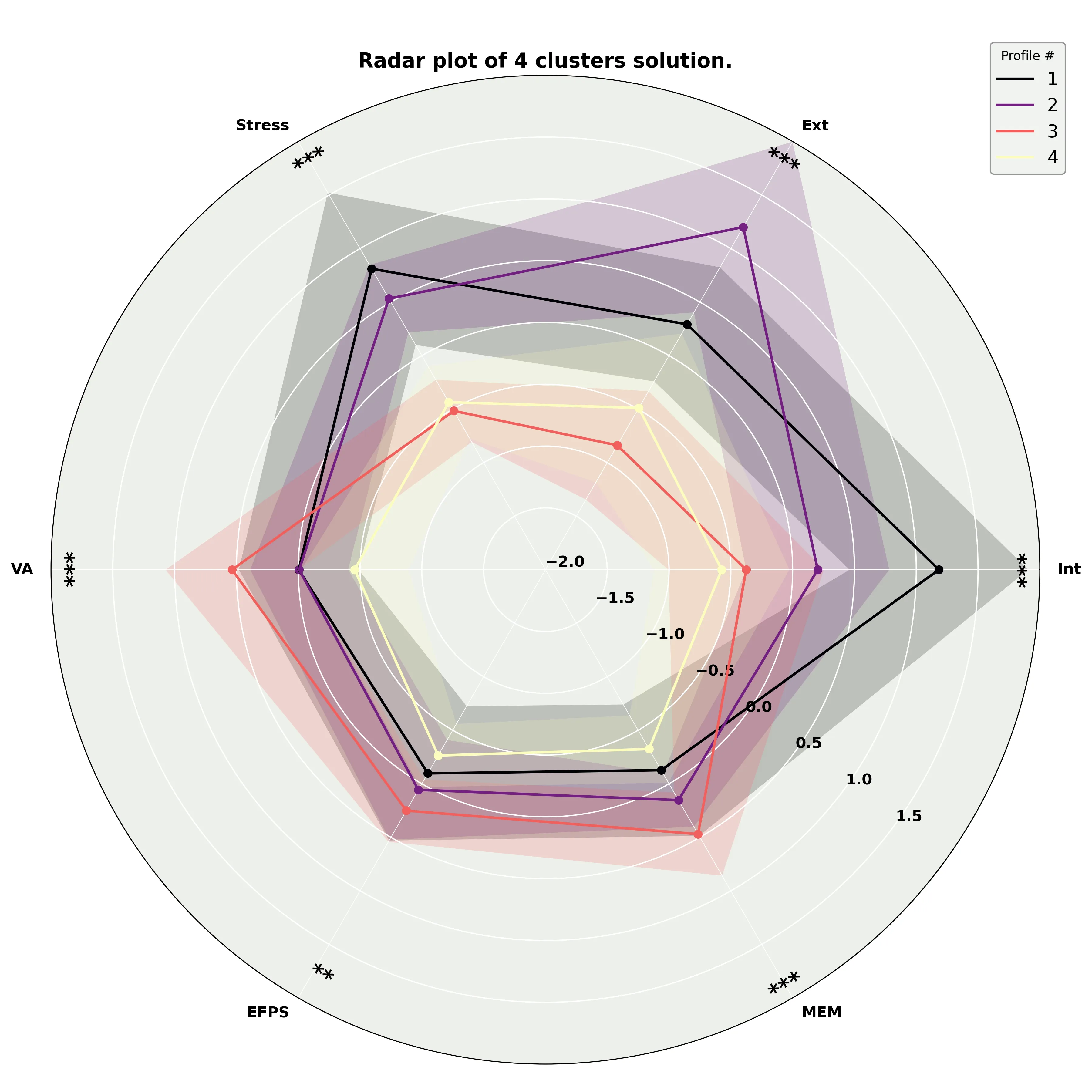
We can see they reproduce the findings from the original paper! That is exactly what we want. Let’s now view the results using a graph network.
Constructing a graph network
To do this, let’s head back into the python console and inspect our new membership values.
from neurostatx.io.loader import DatasetLoader
# Load the output from the previous script.df = DatasetLoader().load_data("testPredictFuzzy/predicted_membership_matrix.xlsx")df.get_data().head(5)
ids Sex Age Int Ext Stress VA EFPS MEM Cluster #1 Cluster #2 Cluster #3 Cluster #40 PC2VLN Female 10.9 0.853711 -0.155164 0.356608 -0.009190 -0.312745 0.046885 0.650611 0.126757 0.103559 0.1190731 XL1LON Male 11.6 0.712829 0.893640 0.629955 0.446043 0.422631 0.336953 0.379016 0.439541 0.104214 0.0772302 F6OQK5 Male 10.7 -0.055407 1.236605 0.501959 -0.657493 -0.451615 -0.343549 0.136026 0.665600 0.076213 0.1221613 TJWBKZ Male 10.3 -0.172911 -1.340310 -0.582634 0.238857 -0.144028 -0.178835 0.090768 0.064187 0.426084 0.4189614 KWQW9D Male 10.8 -0.258481 -0.895303 -0.610380 -0.297869 -0.111272 0.016617 0.050047 0.039926 0.265102 0.644925We can see that the membership values for our four clusters have been appended to the original dataframe!
We can use those membership values to build our graph network. Let’s leverage additional
NeuroStatX function to do so. Most of those functions have been explained in the Introduction to NeuroStatX
section.
from neurostatx.io.loader import GraphLoaderfrom neurostatx.network.utils import get_nodes_and_edges
# Let's drop the descriptive column and original scores.df.drop_columns([i for i in range(1,9)])
# Let's now construct pairs of subject-centroid nodes.pairs, _, _ = df.custom_function(    get_nodes_and_edges)
# Now build our graph.G = GraphLoader().build_graph(    pairs,    "node1",    "node2",    edge_attr="membership")
# Compute the layout.G.layout(weight="membership")
# Let's view this graph.G.visualize(    "predictedsubjects.png",    weight="membership",    edge_width_multiplier=1    )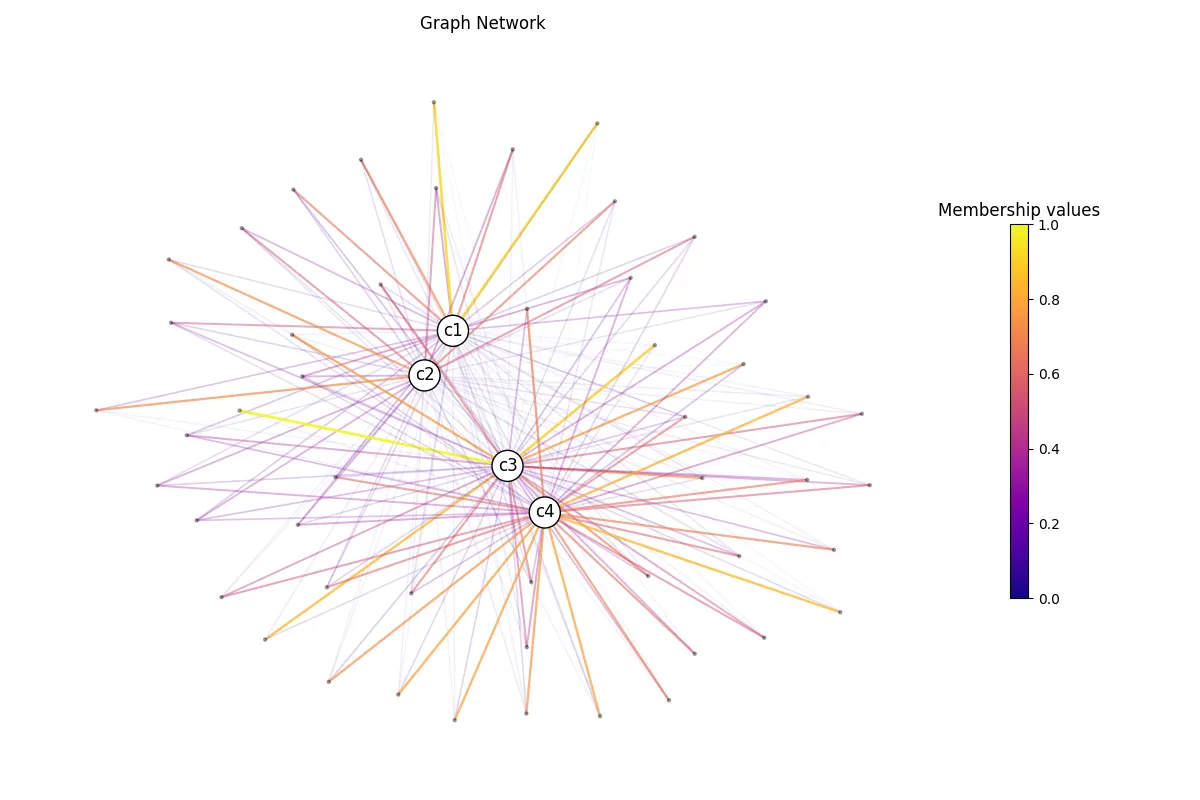
There you go! Obviously, the layout is different than the one presented in Gagnon A. et al. (2025) since we have much less subjects. You are now ready to use those membership values in your statistical analysis!