Introduction to NeuroStatX
Loading and Preparing Data
The NeuroStatX package provides modular data loading utilities for tabular and network-based data
commonly encountered in neurocognitive and connectomic research.
This tutorial introduces the two main loader classes:
DatasetLoaderfor structured behavioral, cognitive, or demographic dataGraphLoaderfor network data (e.g., constructing a graph from fuzzy membership values)
DatasetLoader
The DatasetLoader class is designed to be able to contain tabular-like data
and access various kind of basic information automatically. You can also interact with
the data, apply functions, and save it in multiple formats.
Here is a brief list of the underlying functions:
- Load data from any formats.
- Import data from existing objects.
- Access metadata.
- Join dataset together.
- Save in any formats.
- Apply custom functions.
Basic Usage
To cover the basic usage of the DatasetLoader class, let’s use the data/example.csv
spreadsheet. You can find this dataset on the data/ folder on the
NeuroStatX GitHub.
It contains 50 dummy subjects, with their sex, age, cognitive, and
behavioral scores.
from neurostatx.io.loader import DatasetLoader
# Initialize the loaderdf = DatasetLoader()
# Load the dataframedf.load_data("data/example.csv")
Accessing basic metadata
Our example dataset is currently loaded, we can access some basic information, such as the number of subjects or the number of variables it contains.
print(df.get_metadata()){'nb_subjects': 50, 'nb_variables': 9}Filtering methods
Once loaded, one might be interested in dropping some columns, or extracting only
the descriptive columns from the dataset. The DatasetLoader already have built-in
functions to do this. Let’s start by viewing the top 5 rows of the data.
df.get_data().head(5) ids Sex Age Int Ext Stress VA EFPS MEM0 PC2VLN Female 10.9 0.853711 -0.155164 0.356608 -0.009190 -0.312745 0.0468851 XL1LON Male 11.6 0.712829 0.893640 0.629955 0.446043 0.422631 0.3369532 F6OQK5 Male 10.7 -0.055407 1.236605 0.501959 -0.657493 -0.451615 -0.3435493 TJWBKZ Male 10.3 -0.172911 -1.340310 -0.582634 0.238857 -0.144028 -0.1788354 KWQW9D Male 10.8 -0.258481 -0.895303 -0.610380 -0.297869 -0.111272 0.016617We can see two descriptive columns, Age and Sex. Now, let’s try extracting them.
df.get_descriptive_columns([1,2]).head(5) # Since they are at position 1 and 2 in the columns Sex Age0 Female 10.91 Male 11.62 Male 10.73 Male 10.34 Male 10.8However, they were not removed from the actual dataset, simply extracted.
Let’s truly remove them from the dataset now using the drop_columns() function.
df.drop_columns([1,2])df.get_data().head(5) ids Int Ext Stress VA EFPS MEM0 PC2VLN 0.853711 -0.155164 0.356608 -0.009190 -0.312745 0.0468851 XL1LON 0.712829 0.893640 0.629955 0.446043 0.422631 0.3369532 F6OQK5 -0.055407 1.236605 0.501959 -0.657493 -0.451615 -0.3435493 TJWBKZ -0.172911 -1.340310 -0.582634 0.238857 -0.144028 -0.1788354 KWQW9D -0.258481 -0.895303 -0.610380 -0.297869 -0.111272 0.016617As you can see, they were successfully removed from the dataset! Now you get the basics
for loading and manipulating datasets. In the following tutorials, you will also learn
to apply functions, and use this class to process and organize your data!
Let’s move to the GraphLoader class now.
GraphLoader
The GraphLoader class is a versatile class to load, build, save, and visualize
graph network object. Similarly to the DatasetLoader class, any functions can
be applied to this class, assuming it is designed to run on a graph network object.
Here is a brief list of currently implemented functions:
- Load a graph network from a file in any format.
- Build a graph from an edge list.
- Compute the layout of the graph.
- Add/fetch attributes to nodes or edges.
- Visualize the graph network.
- Save the graph network in any format.
Basic Usage
Since we do not have currently a graph network, let’s build one from scratch, starting
by creating a small dataframe then feeding it to the GraphLoader class.
import pandas as pdfrom neurostatx.io.loader import GraphLoader
# Dummy dataframe containing 3 columns and 3 rows.data = pd.DataFrame({ 'source': ['c1', 'c2', 'c3'], 'target': ['c2', 'c3', 'c1'], 'weight': [0.2, 0.5, 0.7]})
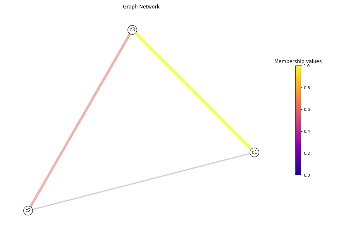
# Build our graph.G = GraphLoader().build_graph(data, edge_attr="weight")We now have a built graph network to play around with! As you can see in the code snippet above, it contains 3 nodes (a, b, c), with three weighted edges (a -> b, b -> c, and c -> a). Now let’s try visualizing it. First, we need to compute a layout, meaning we need to determine where our nodes will be in our network space. There is multiple options to do this, but let’s stick to the default for now (e.g., spring layout). For weighted graph, this allows the relative position of each node to be determined using the edge’s weight.
G.layout(weight="weight")G.visualize("test.png", weight="weight")If you open test.png, you will see your graph network with weight as the
edge color and size!
If you want, you can play around with the visualize() function to get the look
you desire. Here a modified version of the previous graph. Of course, the node positions
will stay the same, since we did not recompute the layout.
G.visualize("test.png", weight="weight", centroid_node_shape=1000, centroid_node_color="lightgray", colormap="viridis", title="Beautiful Graph Network", legend_title="Weight")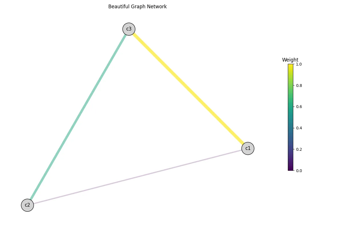
Adding node and edge attributes
An interesting aspect of graph network is that you can append data to both nodes and edges. For example, if nodes are subjects, we could potentially add demographic data such as age to each node. First, let’s look at which data is currently contained within each node.
G.get_graph().nodes(data=True)NodeDataView({'c1': {'pos': [0.9999999999999999, -0.13638075527832896]}, 'c2': {'pos': [-0.9483498360161102, -0.5075132847536213]}, 'c3': {'pos': [-0.05165016398389009, 0.6438940400319502]}})We see that only the node positions is accessible for now. Those came from our previous computation of the graph layout. Let’s now add age to each node and see what happen.
# Create a dictionary of age for each node.age = {    "c1": {"age": 20},    "c2": {"age": 26},    "c3": {"age": 32}}
# Add it to the graph object.G.add_node_attribute(age)G.get_graph().nodes(data=True)NodeDataView({'c1': {'pos': [0.9999999999999999, -0.13638075527832896], 'age': 20}, 'c2': {'pos': [-0.9483498360161102, -0.5075132847536213], 'age': 26}, 'c3': {'pos': [-0.05165016398389009, 0.6438940400319502], 'age': 32}})You can see that each node has now its associated age. To add edge attributes,
you can repeat the previous process but use the add_edge_attributes() function.
Here is a small example.
# Create a dictionary of pair of nodes and the edge attribute.length = {    ("c1", "c2"): {"length": 100},    ("c2", "c3"): {"length": 200},    ("c3", "c1"): {"length": 150}}
# Add it to the graph.G.add_edge_attribute(length)G.get_graph().edges(data=True)EdgeDataView([('c1', 'c2', {'weight': 0.2, 'length': 100}), ('c1', 'c3', {'weight': 0.7, 'length': 150}), ('c2', 'c3', {'weight': 0.5, 'length': 200})])You can even see the previous weight data that we initially set! Now, we could recompute
a graph layout using the length rather than weight, and visualize the results.
# Layout computation.G.layout(weight="length")G.visualize("test_length.png", weight="length")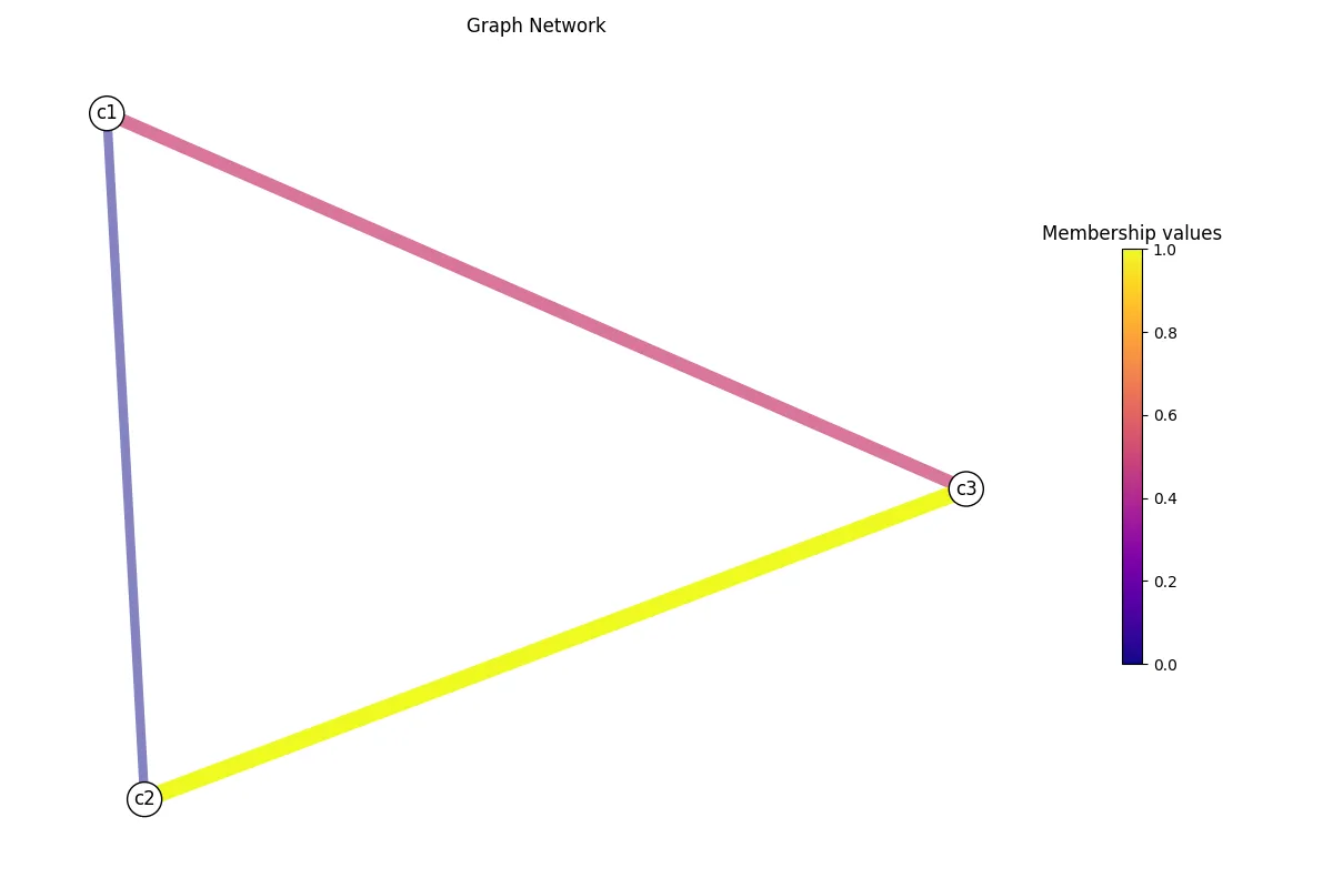
There it is! You recomputed and visualized the graph network using the length
data rather than the weight. Now, you can save your graph network using save_graph(),
and then load it back using load_graph() similarly to the DatasetLoader.